Likelihood Ratio Test for Conditional Variance Models
This example shows how to compare two competing, conditional variance models using a likelihood ratio test.
Step 1. Load the data and specify a GARCH model.
Load the Deutschmark/British pound foreign exchange rate data included with the toolbox, and convert it to returns. Specify a GARCH(1,1) model with a mean offset to estimate.
load Data_MarkPound
r = price2ret(Data);
T = length(r);
Mdl = garch('Offset',NaN,'GARCHLags',1,'ARCHLags',1);
Step 2. Estimate the GARCH model parameters.
Fit the specified GARCH(1,1) model to the returns series using estimate. Return the value of the loglikelihood objective function.
[EstMdl,~,logL] = estimate(Mdl,r);
    GARCH(1,1) Conditional Variance Model with Offset (Gaussian Distribution):

                   Value       StandardError    TStatistic      PValue
                ___________    _____________    __________    __________

    Constant     1.0757e-06     3.5725e-07         3.0112      0.0026021
    GARCH{1}        0.80606       0.013274         60.724              0
    ARCH{1}         0.15311       0.011532         13.278     3.1257e-40
    Offset      -6.1314e-05     8.2867e-05       -0.73991        0.45936
The estimation output shows the four estimated parameters and corresponding standard errors. The t statistic for the mean offset is not greater than two in magnitude, suggesting this parameter is not statistically significant.
Step 3. Fit a GARCH model without a mean offset.
Specify a second model without a mean offset, and fit it to the returns series.
Mdl2 = garch(1,1);
[EstMdl2,~,logL2] = estimate(Mdl2,r);
    GARCH(1,1) Conditional Variance Model (Gaussian Distribution):

                  Value       StandardError    TStatistic      PValue
                __________    _____________    __________    __________

    Constant    1.0535e-06     3.5048e-07        3.0058       0.0026487
    GARCH{1}       0.80657        0.01291        62.478               0
    ARCH{1}        0.15436       0.011574        13.336      1.4293e-40
All the t statistics for the new fitted model are greater than two in magnitude.
Step 4. Conduct a likelihood ratio test.
Compare the fitted models EstMdl and EstMdl2 using the likelihood ratio test. The number of restrictions for the test is one (only the mean offset was excluded in the second model).
[h,p] = lratiotest(logL,logL2,1)
h = logical
   0
p = 0.4534
The null hypothesis of the restricted model is not rejected in favor of the larger model (h = 0). The model without a mean offset is the more parsimonious choice.
Step 5. Infer the conditional variances and standardized innovations.
Infer and plot the conditional variances and standardized innovations for the fitted model without a mean offset (EstMdl2).
v = infer(EstMdl2,r);
inn = r./sqrt(v);

figure
subplot(2,1,1)
plot(v)
xlim([0,T])
title('Conditional Variances')

subplot(2,1,2)
plot(inn)
xlim([0,T])
title('Standardized Innovations')
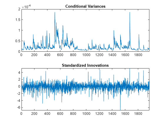
The inferred conditional variances show the periods of high volatility.
See Also
Objects
Functions
estimate|infer|lratiotest
Related Examples
- Specify Conditional Variance Model for Exchange Rates
- Simulate Conditional Variance Model
- Forecast a Conditional Variance Model
More About
You can also select a web site from the following list:
Americas
- América Latina (Español)
- Canada (English)
- United States (English)
Europe
- Belgium (English)
- Denmark (English)
- Deutschland (Deutsch)
- España (Español)
- Finland (English)
- France (Français)
- Ireland (English)
- Italia (Italiano)
- Luxembourg (English)
- Netherlands (English)
- Norway (English)
- Österreich (Deutsch)
- Portugal (English)
- Sweden (English)
- Switzerland
- United Kingdom (English)