Create Black-Box Models of a Robotic Arm System Using Neural Networks

Example System: Industrial Robot Arm

Consider a robot arm described by a nonlinear three-mass flexible model. The input to the robot is the applied torque $$u(t)=\tau (t)$$ generated by the electrical motor. The resulting angular velocity of the motor $$y(t)=\frac{d}{dt}{q}_m(t)$$ is the measured output.

You can derive the equations of motion for this system. For example, a nonlinear state-space description of this system uses five states. For more information on this system, see the example Modeling an Industrial Robot Arm.

The data sets used in this example are saved in robotarmdata.mat.

Prepare Data

Load the data sets, prepare both the estimation and validation data, and downsample the data 10 times for this example.

load robotarmdata.mat
eData = iddata(ye,ue,5e-4,InputName="Torque", ...
    OutputName="Angular Velocity",Tstart=0);
eData = idresamp(eData,[1 10]);
eData.Name = "estimation data"

eData =

Time domain data set with 1984 samples.  
Sample time: 0.005 seconds                
Name: estimation data                     
                                          
Outputs                Unit (if specified)
   Angular Velocity                       
                                          
Inputs                 Unit (if specified)
   Torque                                 
                                          
Data Properties

vData = iddata(yv3,uv3,5e-4,InputName="Torque", ...
    OutputName="Angular Velocity",Tstart=0);
vData = idresamp(vData,[1 10]);
vData.Name = "validation data";
idplot(eData,vData)
legend show

Specify Linear Regressor Object

Specify the input and output names of the regressors.

output_name = "Angular Velocity";
input_name = "Torque";
names = [output_name,input_name];

To choose the correct lags for the regressors, perform a linear estimation based order search using the arxstruc and selstruc commands. Search through all orders in the range 1:10 for the output, 1:10 for the input, and 0:2 for the minimum input delay.

na_range = 1:10;
nb_range = 1:10;
nk_range = 0:2;
NN = struc(na_range,nb_range,nk_range);
V = arxstruc(eData,vData,NN);
selstruc(V)

ans = 1×3

     3     5     0

The dialog box suggests that the orders leading to the best fit with the validation data are na=3, nb=6, and nk=1, where na is the output order, nb is the input order, and nk is the input-output delay. But a slightly smaller order using na=3, nb=5, and nk=0 seems to work almost as well. Select the smaller order values. This choice, where nk=0, implies that the model has feedthrough.

Specify a linear regressor object with output and input regressor sets containing three and five regressors with lags ranging from 1 to 3 and 0 to 4, respectively.

output_lag = 1:3;
input_lag = 0:4;
lags = {output_lag,input_lag};

Create the linear regressor object.

lreg = linearRegressor(names,lags);

Get the regressors used by the model.

getreg(lreg)

ans = 8×1 string
    "Angular Velocity(t-1)"
    "Angular Velocity(t-2)"
    "Angular Velocity(t-3)"
    "Torque(t)"
    "Torque(t-1)"
    "Torque(t-2)"
    "Torque(t-3)"
    "Torque(t-4)"

This linear regressor object is equivalent to the ARX model order matrix [na nb nk]=[3 5 0].

Nonlinear ARX Model Identification

Identify nonlinear ARX models by using different configurations of neural networks for mapping the regressors to the output.

Use Regression Neural Network

First, try a regression neural network. Create a neural network object with one hidden layer of size 5 and one hidden layer of size 3 by using idNeuralNetwork. Set NetworkType to "RegressionNeuralNetwork (Statistics and Machine Learning Toolbox)". Specify the activation function of both the layers as relu.

net1 = idNeuralNetwork([5 3],"relu",NetworkType="RegressionNeuralNetwork");

Prepare training options by setting Focus to "simulation" using nlarxOptions. This setting is to help the model perform well for long horizon predictions and amounts to training the network in a recurrent (closed-loop) configuration. Estimate the nonlinear ARX model that uses net1 as the output function using nlarx. Set the random number generator seed for reproducibility.

rng default
opt = nlarxOptions(Focus="simulation",Display="on");
nlarx1 = nlarx(eData,lreg,net1,opt)

nlarx1 =

Nonlinear ARX model with 1 output and 1 input
  Inputs: Torque
  Outputs: Angular Velocity

Regressors:
  Linear regressors in variables Angular Velocity, Torque
  List of all regressors

Output function: Regression neural network
Sample time: 0.005 seconds

Status:                                                     
Estimated using NLARX on time domain data "estimation data".
Fit to estimation data: 75.05% (simulation focus)           
FPE: 1.169, MSE: 27                                         

Model Properties

Use Deep Learning Network

Next, create a deep learning network object that contains three hidden layers using idNeuralNetwork. Specify that the first hidden layer uses 10 units of the tanh activation function, the second hidden layer uses 5 units of the sigmoid activation function, and the last layer uses 2 units of the gelu activation function.

LayerSizes = [10 5 2];
net2 = idNeuralNetwork(LayerSizes,["tanh","sigmoid","gelu"],NetworkType="dlnetwork");

To speed up the training, split the data into segments of 500 samples each with no overlap.

eDataSplit = utSegmentData(eData,500,500);

Use Levenberg-Marquardt as the search method with a maximum of five iterations. Estimate the nonlinear ARX model with net2 as the output function using nlarx.

opt.SearchMethod = "lm";
opt.SearchOptions.MaxIterations = 5;
nlarx2 = nlarx(eDataSplit,lreg,net2,opt)

nlarx2 =

Nonlinear ARX model with 1 output and 1 input
  Inputs: Torque
  Outputs: Angular Velocity

Regressors:
  Linear regressors in variables Angular Velocity, Torque
  List of all regressors

Output function: Deep learning network
Sample time: 0.005 seconds

Status:                                                       
Estimated using NLARX on time domain data "estimation data".  
Fit to estimation data: [67.8 19.65 72.36]% (simulation focus)
FPE: 1.264, MSE: [36.23 23.83 26.15]                          

Model Properties

Compare the model fit to the original, unsegmented estimation data.

compare(eData,nlarx2)

Use Shallow Network

You can also use shallow networks to represent the neural network function map. Create a feedforward (shallow) network that uses three hidden layers of size 4, 6, and 1 using feedforwardnet (Deep Learning Toolbox). The network uses the tanh activation function.

snet = feedforwardnet([4 6 1]);

Incorporate the shallow network into the idNeuralNetwork object net3.

net3 = idNeuralNetwork(snet);

Use lsqnonlin as the search method with a maximum of 20 iterations. Estimate the nonlinear ARX model with net3 as the output function using nlarx.

opt.SearchMethod = "lsqnonlin";
opt.SearchOptions.MaxIterations = 20;
nlarx3 = nlarx(eData,lreg,net3,opt)

nlarx3 =

Nonlinear ARX model with 1 output and 1 input
  Inputs: Torque
  Outputs: Angular Velocity

Regressors:
  Linear regressors in variables Angular Velocity, Torque
  List of all regressors

Output function: Shallow network of Deep Learning Toolbox
Sample time: 0.005 seconds

Status:                                                     
Estimated using NLARX on time domain data "estimation data".
Fit to estimation data: 75.56% (simulation focus)           
FPE: 1.084, MSE: 25.91                                      

Model Properties

Check the model performance for infinite-step-ahead prediction on the validation data set by comparing the fit accuracies for the models nlarx1, nlarx2, and nlarx3.

compare(vData,nlarx1,nlarx2,nlarx3)

Hammerstein-Wiener Model Identification

Identify Hammerstein-Wiener models by using different configurations of neural networks for mapping the regressors to the output.

Use Regression Neural Network

Create a regression neural network object with one hidden layer of size 5 and one hidden layer of size 7 using idNeuralNetwork. Specify the activation function of both the layers as sigmoid.

net4 = idNeuralNetwork([5 7],"sigmoid",NetworkType="RegressionNeuralNetwork");

Estimate the Hammerstein-Wiener model with no input nonlinearity and net4 as the output nonlinearity using nlhw. Specify the model order as [3 5 0] based on the selstruc analysis performed earlier. Here, nf is similar to the na order of an ARX model.

nb = 5;
nf = 3;
nk = 0;
nlhw1 = nlhw(eData,[nb,nf,nk],[],net4)

nlhw1 =

Hammerstein-Wiener model with 1 output and 1 input

Linear transfer function corresponding to the orders nb = 5, nf = 3, nk = 0

Input nonlinearity: None
Output nonlinearity: Regression neural network
Sample time: 0.005 seconds

Status:                                                    
Estimated using NLHW on time domain data "estimation data".
Fit to estimation data: 76.4%                              
FPE: 25.9, MSE: 24.16                                      

Model Properties

Use Deep Learning Network

Create a deep learning network object that contains one hidden layer of size 8, one hidden layer of size 5, and one hidden layer of size 3 using idNeuralNetwork. Specify the activation function of all three layers as leakyRelu.

net5 = idNeuralNetwork([8 5 3],"leakyRelu",NetworkType="dlnetwork");

Estimate the Hammerstein-Wiener model with no input nonlinearity and net5 as the output nonlinearity using nlhw. Specify the same model order as before.

nlhw2 = nlhw(eData,[nb,nf,nk],[],net5)

nlhw2 =

Hammerstein-Wiener model with 1 output and 1 input

Linear transfer function corresponding to the orders nb = 5, nf = 3, nk = 0

Input nonlinearity: None
Output nonlinearity: Deep learning network
Sample time: 0.005 seconds

Status:                                                    
Estimated using NLHW on time domain data "estimation data".
Fit to estimation data: 75.76%                             
FPE: 27.96, MSE: 25.48                                     

Model Properties

Use Shallow Network

Create a cascade-forward (shallow) network with one hidden layer of size 10 using cascadeforwardnet (Deep Learning Toolbox).

net = cascadeforwardnet(10);

Incorporate the shallow network into the idNeuralNetwork object net6.

net6 = idNeuralNetwork(net);

Estimate the Hammerstein-Wiener model with no input nonlinearity and net6 as the output nonlinearity using nlhw. Specify the same model order as before.

nlhw3 = nlhw(eData,[nb,nf,nk],[],net6)

nlhw3 =

Hammerstein-Wiener model with 1 output and 1 input

Linear transfer function corresponding to the orders nb = 5, nf = 3, nk = 0

Input nonlinearity: None
Output nonlinearity: Shallow network of Deep Learning Toolbox
Sample time: 0.005 seconds

Status:                                                    
Estimated using NLHW on time domain data "estimation data".
Fit to estimation data: 76.98%                             
FPE: 23.95, MSE: 22.98                                     

Model Properties

Check the model performance for infinite-step-ahead prediction on the validation data set by comparing the fit accuracies for the models nlhw1, nlhw2, and nlhw3.

compare(vData,nlhw1,nlhw2,nlhw3)

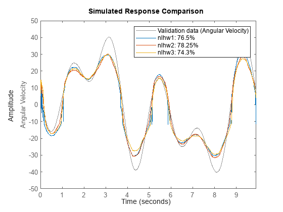
The plots in this example show that the black-box models created using neural networks have a good fit percentage and perform well for longer prediction horizons.