Model an Anti-Lock Braking System
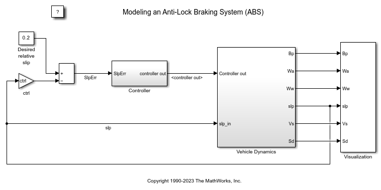
This example shows how to model a simple Anti-Lock Braking System (ABS). The model simulates the dynamic behavior of a vehicle under hard braking conditions. The model represents a single wheel, which may be replicated a number of times to create a model for a multi-wheel vehicle.
This model uses the signal logging feature in Simulink®. The model logs signals to the MATLAB® workspace, where you can view and analyze them. View the code in the ModelingAnAntiLockBrakingSystemExample.m file to see how the software logs the signals.
In the sldemo_absbrake model, the wheel speed is calculated in a separate model named sldemo_wheelspeed_absbrake. This component is then referenced using a Model block. Both the top model and the referenced model use a variable-step solver, so Simulink will track zero crossings in the referenced model.
Model Physics
The wheel rotates with an initial angular speed that corresponds to the vehicle speed before the brakes are applied. The model uses separate integrators to compute wheel angular speed and vehicle speed. The model uses two speeds to calculate slip, which is determined by Equation 1. Note that vehicle speed is expressed as an angular velocity.

Equation 1


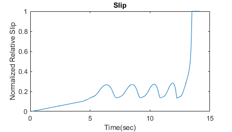
Slip is zero when wheel speed and vehicle speed are equal, and slip equals one when the wheel is locked. A desirable slip value is 0.2, which means that the number of wheel revolutions equals 0.8 times the number of revolutions under nonbraking conditions with the same vehicle velocity. This value maximizes the adhesion between the tire and road and minimizes the stopping distance with the available friction.
Model Analysis
The friction coefficient between the tire and the road surface, mu, is an empirical function of slip, known as the mu-slip curve. The software creates mu-slip curves by passing MATLAB variables into the block diagram using a Simulink lookup table. The model multiplies the friction coefficient, mu, by the weight on the wheel, W, to yield the frictional force, Ff, acting on the circumference of the tire. Ff is divided by the vehicle mass to produce the vehicle deceleration, which the model integrates to obtain vehicle velocity.
The model uses an ideal anti-lock braking controller that uses bang-bang control based upon the error between actual slip and desired slip. The desired slip is set to the value of slip at which the mu-slip curve reaches a peak value, which is the optimum value for minimum braking distance.
In an actual vehicle, the slip cannot be measured directly, so this control algorithm is not practical. This example uses the alogirithm to illustrate the conceptual construction of such a simulation model.
Double-click the Wheel Speed subsystem to open it. Given the wheel slip, the desired wheel slip, and the tire torque, this subsystem calculates the wheel angular speed.
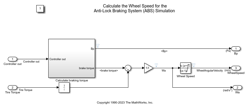
To control the rate of change of brake pressure, the model subtracts actual slip from the desired slip and feeds this signal into a bang-bang control (+1 or -1, depending on the sign of the error). This on/off rate passes through a first-order lag that represents the delay associated with the hydraulic lines of the brake system. The model then integrates the filtered rate to yield the actual brake pressure. The resulting signal, multiplied by the piston area and radius with respect to the wheel (Kf), is the brake torque applied to the wheel.
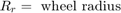
The model multiplies the frictional force on the wheel by the wheel radius (Rr) to give the accelerating torque of the road surface on the wheel. The brake torque is subtracted to give the net torque on the wheel. Dividing the net torque by the wheel rotational inertia I yields the wheel acceleration, which is then integrated to provide wheel velocity. In order to keep the wheel speed and vehicle speed positive, the model uses limited integrators.
Simulate in ABS Mode
On the Simulation tab, click Run to run the simulation. You can also run the simulation by entering the sim('sldemo_absbrake') command in the MATLAB Command Window. ABS is turned on during this simulation.
The model logs relevant data to MATLAB workspace in a structure called sldemo_absbrake_output. Logged signals have a blue indicator. In this case yout and slp are logged.
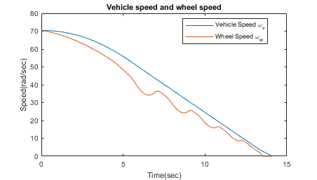
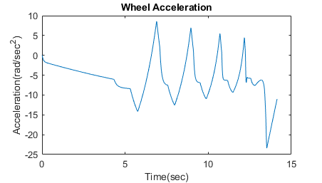
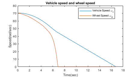
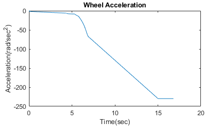
These plots show the ABS simulation results for default parameters. The first plot shows the wheel angular velocity and corresponding vehicle angular velocity. The second plot shows that the wheel speed stays below vehicle speed without locking up, with vehicle speed going to zero in less than 15 seconds. Wheel acceleration, Wheel slip ratio and braking pressure are monitored. Wheel slip ratio is used to determine whether the wheel is locked or not. Braking cycles are observed by monitoring stopping distance and braking pressure.
Simulate Without ABS
For more meaningful results, consider the vehicle behavior without ABS. In the MATLAB Command Window, set the model variable ctrl = 0. This setting disconnects the slip feedback from the controller, resulting in maximum braking.
Run the simulation again to model braking without ABS.
Braking with ABS Versus Braking Without ABS
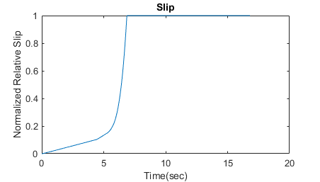
In the plot showing vehicle speed and wheel speed, observe that the wheel locks up in about seven seconds. The braking, from that point on, is applied in a suboptimal part of the slip curve. That is, when slip = 1, as the slip plot shows, the tire skids so much on the pavement that the friction force drops off.
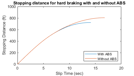
This plot shows the distance traveled by the vehicle for the two cases. Without ABS, the vehicle skids about an extra 100 feet, taking about three seconds longer to come to a stop.
Extended Modeling
The controller in this example is idealized, but you can use any control algorithm in its place to evaluate the performance of your system. For rapid prototyping of the proposed algorithm, you can also use Simulink Coder™.
Simuink Coder generates and compiles C code for the controller hardware to test the concept in a vehicle. This process significantly reduces the time needed to prove new ideas by enabling actual testing early in the development cycle.
For a hardware-in-the-loop braking system simulation, Simulink Coder allows you to generate real-time C code to remove the bang-bang controller and run the equations of motion on real-time hardware to emulate the wheel and vehicle dynamics. You can then test an actual ABS controller by interfacing it to the real-time hardware, which runs the generated code. In this scenario, the real-time model would send the wheel speed to the controller, and the controller would send brake action to the model.
Related Topics
You can also select a web site from the following list:
Americas
- América Latina (Español)
- Canada (English)
- United States (English)
Europe
- Belgium (English)
- Denmark (English)
- Deutschland (Deutsch)
- España (Español)
- Finland (English)
- France (Français)
- Ireland (English)
- Italia (Italiano)
- Luxembourg (English)
- Netherlands (English)
- Norway (English)
- Österreich (Deutsch)
- Portugal (English)
- Sweden (English)
- Switzerland
- United Kingdom (English)